From heat to hidden frequencies: Understanding the Fourier Transform

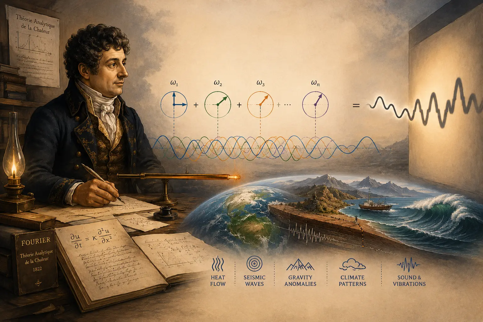
"Education is the ability to listen to almost anything without losing your temper or your self-confidence."

Quick disclosure before anything else: I am not a mathematician. I have a physics background and roughly a decade of quietly Googling things I should have understood the first time somebody explained them to me. If you're expecting a confident expert walking you through an elegant idea with total command of the material, I have to warn you now that is not this article is. What I can offer instead is the story of someone who used a very famous piece of mathematics for years without understanding it even a little, followed by what happened when he finally sat down and forced himself to actually get it.

If that sounds like your relationship with roughly half the equations you memorized for an exam and immediately forgot, we might get along quite nicely. You don't need to know any signal processing to understand what I am going to discuss next. You don't need to remember trigonometry fondly, or at all. You just need to be willing to follow one idea at a time, because that's genuinely all this is, one idea, then the next one it quietly makes necessary, then the next.

I arrived at my masters DSP class from a physics background, having never formally studied signal processing before, and did what a lot of people do with a subject that feels intellectually interesting but somehow personally distant: I learned it well enough to survive the exam, and not a page more. At the time, the Fourier Transform felt like one more mathematical technique. Useful, probably. Examinable, certainly. Not something I expected to still be thinking about a decade and several job titles later.

I could not have been more wrong. Though, in my defense, being wrong about which subjects will matter later is basically the entire graduate experience.

Years of faking it

There's something strange about learning a thing under duress, for one exam, filed mentally under "not mine." You often only discover how important it actually was after it has spent years quietly rearranging your work behind your back. That's exactly what happened here. The Fourier Transform never announced itself. It just kept turning up like a landlord who shows up unannounced, except instead of asking for rent, just sort of solve my problem and leave without explaining.

It followed me into my PhD, hiding inside lithospheric flexure and gravity modelling. It followed me into seismic processing. Then bathymetric roughness analysis. Then it kept on following me into all domains I tried to escape into. And then, much later, it followed me home, literally, in the shape of a piece of software called REDFIT. My wife works with micropaleontology records that are, almost without exception, sampled maddeningly unevenly across time, and REDFIT is the standard tool for coaxing a frequency spectrum out of exactly that kind of data. Her own training, in palaeontology, had never once required her to sit through a signal processing course. So one evening the Fourier Transform ended up back at our dinner table, anyway, this time in the entirely domestic form of me trying to explain what a 'power spectrum' actually is to someone who, quite reasonably, just wanted to know whether her sediment record had a cycle in it or not.

What eventually got under my skin wasn't that the Fourier Transform was everywhere. It was the slow, mildly uncomfortable realization that despite using it constantly, I had never actually understood it. I knew how to summon it. I could type fft(signal) with the total, unearned confidence of a man who knows exactly which button does what and none of why it works. I knew which menu option to click. I knew which commands to run. And every so often, something would go sideways in a way that made it very clear I wasn't actually in control of anything. The inverse transform wouldn't reconstruct what I expected. The spectrum would show strange mirror images I couldn't explain. Filtering would introduce artefacts out of nowhere. Two pieces of software would quietly disagree with each other about normalization, like students who both insist they're right and refuse to compare notes. The code worked. Until it didn't. And every time it didn't, I discovered, a little painfully, that I understood the software far, far better than I understood the mathematics sitting underneath it.

The turning point was a YouTube animation. I want to be honest about how unglamorous this moment was too: I didn't have an epiphany in a lecture hall, or while reading a paper, or during some quiet moment of scholarly reflection. I had it at around 1 AM, procrastinating instead of finishing a report I was already late on, watching a video of dots going around in circles, the exact kind of thing YouTube recommends once it has correctly identified you as someone who will click on literally anything with a satisfying visual.

A single point moved around a circle at a steady pace. Its shadow, cast onto a line beside it, traced a smooth back-and-forth wiggle. Then a second rotating point was added, spinning at a different speed. Then a third. Different speeds, different sizes, different starting positions, and slowly, out of nothing but circles going around and around, shapes started appearing that had no business looking the way they did. Square waves. Sawtooth waves. Jagged, complicated curves that looked nothing like a circle should be capable of producing. For the first time, I stopped seeing the Fourier Transform as a computational chore I ran, and started seeing it as a way of actually looking at nature. That was the moment it became beautiful instead of merely useful.

It helped, a little later, to learn I wasn't the only one who'd needed convincing. When Joseph Fourier first proposed that pretty much any function, any curve, however jagged, however odd, could be built entirely out of sums of simple sine and cosine waves, some of the sharpest mathematicians alive at the time thought he'd lost the plot. Heavyweights like Joseph-Louis Lagrange, Pierre-Simon Laplace, and Siméon Denis Poisson pushed back hard. Lagrange, in particular, was stubbornly convinced that smooth, rolling waves could never model a line with sharp corners. It was too bold. Too elegant to possibly be true. Which is, honestly, a small comfort: if the literal namesakes of half our math textbooks needed convincing, I feel slightly less embarrassed about needing around ten years to get there myself. History eventually sided firmly with Fourier, the same basic idea now quietly underwrites acoustics, quantum mechanics, image processing, astronomy, medical imaging, communications, machine learning, and, closer to home, an enormous amount of geophysics.

If you work in geoscience, in fact, you've almost certainly already shaken hands with the Fourier Transform, whether you noticed or not. Every time you filter a seismic trace. Every time you analyse a gravity or magnetic anomaly. Every time you examine how topography changes across different wavelengths, or compute a power spectrum, or go looking for periodicity buried in a climate record, or smooth a noisy raster because it looks like it's been attacked by static. The Fourier Transform is back there in the machinery, invisible, quietly doing the actual work, while you get to take all the credit in the results section.

So here, we start with the problem: a genuinely mundane, practical one. If it works, by the time we get to the actual Fourier Transform, near the end, it should feel less like a formula somebody is asking you to accept on faith, and more like something you'd have arrived at yourself eventually, just slower, and with more swearing.

Let's begin, then, exactly where Fourier did. Not with oscillations, not with frequency, not even with mathematics, but with a question that sounds almost embarrassingly ordinary: how does heat move through a metal rod?

A hot metal rod and an unexpected question

It's easy to forget that the Fourier Transform wasn't invented for seismic data, or gravity anomalies, or climate records, or oscillations of any kind. It came out of a much less glamorous question: how does heat travel through a solid object?

Heat a spoon in a cup of tea, and eventually the handle gets warm too. Stick one end of an iron rod into a fire, and eventually the other end warms up as well. These are the kinds of observations so mundane that today nobody ever pauses mid-conversation to marvel at them. Two centuries ago, though, this exact question was one of the defining scientific problems of the age. Because the early 1800s saw the beginning of the industrial revolution, large machinery that ran on heat, and occasionally, sometimes catastrophically, did not handle it well. Steam engines. Iron bridges. Furnaces and boilers running at a scale nobody had built for before. Heat decided whether all of that worked reliably or exploded, which is the sort of environment that focuses the mind on the question "how does heat actually move through metal, precisely?"

Picture a blacksmith with one end of a long iron bar resting in the forge. That end glows almost immediately, orange giving way to white. The far end remains stubbornly cool enough to hold with a bare hand. Between them lies a continuously changing temperature gradient: every point along the rod has its own temperature, and every one of those temperatures is constantly changing. A point that's cool now may be warm in five minutes. A point that's already hot may continue heating or begin cooling, depending entirely on what's happening nearby.

That, stripped of all the later fame, was Fourier's original problem.

Heat flows from warmer regions to cooler ones, gradually smoothing temperature differences. Given enough time, the entire rod settles into a single, uniform temperature.

Imagine the temperature isn't simply hot at one end and cool at the other. Instead, picture alternating narrow bands of hot and cold packed closely together, alongside broad, gentle changes spread over much greater distances. Now if we measure what happens, the narrow bands disappear rapidly because heat needs to travel only a short distance to erase the contrast. The broader variations evolve much more slowly because heat must diffuse across a much larger distance.

Long before Fourier wrote down a single equation, the iron rod was already behaving like a filter, removing fine-scale temperature variations while preserving the larger ones. In modern language, we would say it damps high spatial frequencies much faster than low ones. The rod is doing signal processing, quietly and effortlessly, simply by being a rod.

Fourier eventually captured this behaviour in what we now call the heat equation:

$$\frac{\partial T}{\partial t} = \kappa \frac{\partial^2 T}{\partial x^2}$$

where \(T\) is temperature, \(x\) is position along the rod, \(t\) is time, and \(\kappa\) is the thermal diffusivity of the material which is a number describing how eagerly heat spreads through it. I promise this looks scarier than it is. Translated into plain English, the left side is asking, "how fast is the temperature changing right now, at this point?" The right side is asking, "how sharply is the temperature curve bending, in space, at this point?" Which means the whole equation is really just saying something profound: Wherever the temperature curve bends sharply, things change fast. Wherever it's gentle, things change slowly. Nature has quietly wired spatial curvature straight into how fast time moves things along, which is to me, a very insightful statement about the universe.

But writing down the heat equation was only half the battle. The equation tells us how temperature changes, not what the temperature will actually be. Suppose I hand you the temperature along the entire rod right now. What will it look like one minute later? Ten minutes later? An hour later? Answering those questions means solving the equation. The symbol \(T\) in the heat equation is not a single temperature reading. It represents the entire temperature distribution along the rod. It is a function of both position and time. Solving the heat equation therefore means finding a mathematical function that satisfies the equation: one that tells us the temperature at every point along the rod, at every instant into the future.

To actually solve this equation, Fourier needed functions that behaved predictably when you differentiated them, because the equation itself has a second derivative sitting right there in it, and any candidate solution needs to survive being differentiated twice without turning into something unrecognisable. This next bit is worth sitting with for a moment, because almost everything later in this article leans on it.

Nothing escapes the family. Nothing new gets invented along the way. The function hasn't morphed into something foreign; it's just been rescaled, flipped in sign, nothing more. And that is precisely the physical fact that makes sine waves useful as building blocks for the heat equation: each one can evolve entirely on its own terms, weakening in place as heat diffuses through the rod, without ever deforming into some other shape or bleeding into some other wavelength. Its shape survives untouched from start to finish. Only its amplitude shrinks, the way a sound fades without ever changing pitch. Which is, frankly, more emotional stability than I managed to display during most of my own household disagreements.

This is what led Fourier to a genuinely audacious claim. If a single sine wave behaves this elegantly under the heat equation, what if every possible temperature distribution, however lumpy, however irregular, could be built entirely by adding up many sine waves, each one evolving completely independently, each one gradually weakening on its own private schedule? Instead of wrestling with one impossibly complicated problem, you solve a pile of very simple ones and just add the answers together at the end. It is rather like untangling a hopelessly knotted ball of string by patiently separating one strand at a time.

There is, however, one huge complication. Even granting Fourier's extraordinary claim, another question shows up immediately. Suppose someone hands you a completely arbitrary signal: a gravity profile, a seismic trace, a temperature curve, anything. How, exactly, is anyone supposed to figure out which sine waves are hiding inside it?

The circle hiding behind every wiggly line

Most of us first meet sine and cosine in a trigonometry classroom, memorising identities, solving triangles, calculating angles, and passing exams without ever being told why any of it might matter again. Years later, when the Fourier Transform shows up, those exact same functions suddenly become the entire foundation of signal processing, and the connection between "thing I memorised for a test" and "thing that apparently runs half of modern science" feels genuinely mysterious. For me, it stayed mysterious for years. The shift only happened once I stopped thinking of sine waves as equations and started thinking of them as motion.

Picture a point travelling around a circle at a constant speed, never speeding up, never slowing down, just going round and round forever. Put a screen beside the circle and watch only the point's vertical position. It drifts up, slides back through the middle, swings down, and comes back, smoothly, predictably, endlessly. That motion, on its own, isn't a sine wave yet. It's just an oscillation: back and forth, back and forth. The wave only appears once we let some other quantity march forward steadily. It can be time, most naturally, but it could just as easily be distance along a survey line, depth down a borehole, or age within a sediment core; the mathematics genuinely doesn't care, and plot the point's changing vertical position against that. The wave is the history of the shadow, not the shadow itself.

Spin the point faster, and the oscillation repeats more often, the frequency goes up. Spin it slower, frequency drops. Move the point farther from the centre, and the swing gets bigger, amplitude increases. Start the rotation from a different point on the circle, and the whole thing kicks off at a different moment, the phase shifts. Three words that sound intimidating enough to belong on a difficult exam — frequency, amplitude, phase — turn out to be nothing more than the plain geometric consequences of something going around in a circle. Once you see it this way, it's genuinely hard to unsee.

Now add a second rotating point, spinning at a different speed, starting from a different angle on its own circle. Its shadow looks different from the first. Add a third. A fourth. Sum all of them together, and the resulting curve gets complicated, while every single ingredient stays perfectly, boringly simple, each one just the shadow of a point going around and around. This is the seed of Fourier's entire idea: maybe a complicated signal isn't fundamentally complicated at all. Maybe it just looks that way because several simple oscillations are happening at once, layered on top of each other. It's the same trick a musical chord pulls on our ears: one rich, unified sound that's secretly several individual notes stacked together, each one perfectly recoverable if we know what we're listening for.

That question sits right at the heart of Fourier analysis. Before we let a computer answer it, we must try answering it ourselves.

Catching one wave red-handed

Suppose someone hands you a gravity profile, and you have a hunch it's hiding an oscillation with a wavelength of roughly 100 kilometres. How would you even start checking?

The obvious idea is very simple: build your own oscillation at exactly that wavelength, lay it directly over the measured signal, and see whether the peaks and troughs line up. Good match! Then maybe that wavelength is really there. Bad match, maybe it isn't. It sounds too basic to count as real science, and yet it is, genuinely, the entire spirit of Fourier analysis in miniature.

Of course, eyeballing two overlapping squiggly lines is not a measurement. It's a vibe, and two people staring at the exact same plot can walk away with two completely different opinions, which is a fine way to have an argument and a terrible way to run an analysis. We need an actual number, not a feeling.

There's also a second, sneakier complication lurking here. Take two oscillations with identical amplitude and identical wavelength, but let one of them start slightly later than the other. Their peaks no longer line up. Compared directly, they look like they disagree, even though they're literally the same oscillation, just shifted along a little. This shift has a proper name: phase.

Actually, to pin an oscillation down completely, we need answers to three separate questions:

1. Does this frequency exist in the signal at all?

2. How large is its amplitude?

3. Where, exactly, does it begin?

The first question alone was never going to be enough. Which is genuinely a little discouraging on first glance because for any given frequency, there are infinitely many possible starting points and amplitudes. Surely we're not expected to test every single one of them?

We're not, thankfully. But before we get to see the way out, we first need a way to measure "resemblance" between two wiggly curves using nothing but arithmetic.

When similarity becomes a number

A computer doesn't see a waveform at all. It sees a list of numbers, full stop, and treats those numbers with exactly the same enthusiasm it treats a grocery list. If we want a machine to recognise an oscillation that agrees with another oscillation, we first have to teach in plain arithmetic what "agreement" even means.

There is a surprisingly simple move. Take the two signals, multiply them together point by point, and add up all the products. At first this looks almost arbitrary, why multiplication, of all operations, and why addition afterward? The answer becomes obvious once you look at what multiplication is quietly doing under the hood. If both signals happen to be positive at the same location, their product is positive. If both happen to be negative at the same spot, the product is still positive. Whenever the two signals move together, in the same direction, they reinforce one another. But if one is positive while the other is negative, the product goes negative, instead of reinforcing, they start actively cancelling each other out. Multiplication, has quietly become a detector of agreement. Points that resemble each other contribute something positive. Points that disagree contribute something negative. Add it all up, and you're left holding a single, honest number.

However, I'm quite confident that anyone who's been paying even loose attention till now, will be starting to feel suspicious again. Compare two oscillations that share exactly the same frequency and exactly the same amplitude, differing only in that one of them starts from a different position than the other. Their peaks no longer line up quite as neatly. Some of the positive contributions vanish. Some new negative ones creep in. The similarity score drops, even though fundamentally, nothing has actually changed about either oscillation. Only their starting positions differ. Our little detector, it turns out, is sensitive not just to frequency, but to phase also.

This leaves us with an uncomfortable new problem: how do we reliably detect a frequency when we don't know its phase ahead of time, short of comparing the signal against infinitely many shifted copies of the same wave, which sounds, frankly, hopeless?

Fortunately, one of the more elegant ideas in all of mathematics lets us dodge that infinite search entirely. And it starts with an observation about two very familiar functions: sine and cosine.

The phase problem (and how to dodge infinity)

If the oscillation hiding inside the signal happens to start at a different position than our reference, the comparison gets worse, even though nothing is actually wrong with either the frequency or the signal. The two oscillations are simply out of step with each other. They differ only in phase.

At first, this looks like a serious dead end. Imagine a signal that genuinely contains an oscillation of some particular frequency, we just don't know where, exactly, it begins. Every possible starting position is a different phase, and since phase can take on infinitely many values, we seem to be staring down an alarming conclusion: for every single frequency we want to check, do we really need to test it against infinitely many phase-shifted versions of the reference wave? If so, this whole approach is dead on arrival.

Before we solve that, it's worth pausing to ask a more basic question: why do we even care this much about frequency in the first place? What is frequency actually telling us?

Now, back to the phase problem. The problem was never that the mathematics failed. The problem is that we only picked one single reference wave and tried to make it describe every possible phase on its own. That was always asking too much of one function.

Here's where the rotating circle earns its keep again. When our rotating point completes one full lap, we can track either its horizontal position or its vertical position, and those two traces differ only in where they begin. When one hits its peak, the other is passing straight through zero. One is a cosine. The other is a sine. Together, they're just the same circular motion, viewed from two directions at right angles to each other.

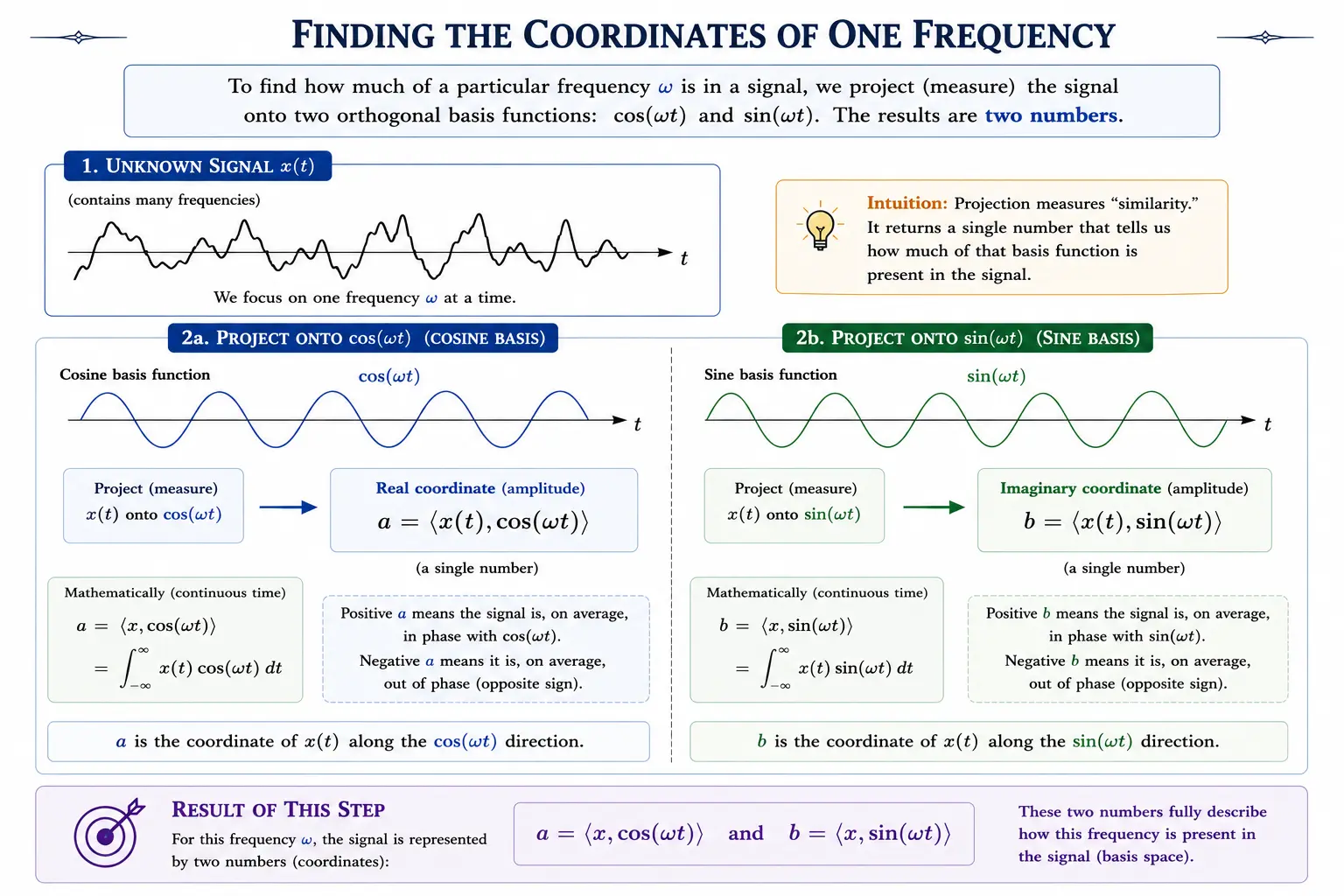
This small geometric fact quietly solves the whole problem. If an oscillation doesn't line up perfectly with our cosine reference, instead of hunting for yet another shifted cosine wave, we can ask a completely different pair of questions: how much of this oscillation resembles a cosine? And how much resembles a sine? It turns out those two questions are enough, genuinely, completely enough. Every possible phase, no matter what it is, can be described as some particular combination of these two fixed reference waves. Instead of searching through infinitely many shifted oscillations, we only ever need to measure two quantities: one cosine coefficient, one sine coefficient. The infinite search just quietly evaporates.

Collapsing infinity into two coordinates

Here's something that looks almost like a paradox: phase can take on infinitely many values, and yet we just claimed that two fixed reference waves, one cosine, one sine, are enough to represent every single one of them. How can two functions possibly stand in for infinity?

Fourier analysis is doing exactly this. For any single frequency, the infinitely many possible phase-shifted versions of the wave were never actually infinite different functions. They're all just different combinations of one fixed cosine and one fixed sine. Instead of inventing a brand-new basis wave for every possible phase, we keep the basis locked in place and let two coefficients absorb all the variation.

And we don't guess those two coefficients. We measure them, using exactly the projection trick from a little earlier. Compare the signal against the cosine reference: that gives you the cosine coefficient. Compare it against the sine reference: that gives you the sine coefficient. Two measurements, two numbers, and between them, the amplitude and phase of the hidden oscillation are pinned down completely, nothing approximated, both numbers pulled directly out of the data itself.

There's an obvious worry worth addressing here, though. If the signal has a strong cosine-like component, wouldn't some of that accidentally leak into the sine measurement too, muddying both numbers at once? It doesn't, sine and cosine are orthogonal, which is the same non-interference we just saw with east and north, dressed up in different clothes. Compare a pure cosine wave against a sine wave of the same frequency over a full cycle, and their positive and negative agreements cancel out perfectly; the similarity score comes out to exactly zero. Each measurement responds only to its own reference wave, with no cross-contamination whatsoever, which is more than I can say for most of my group projects.

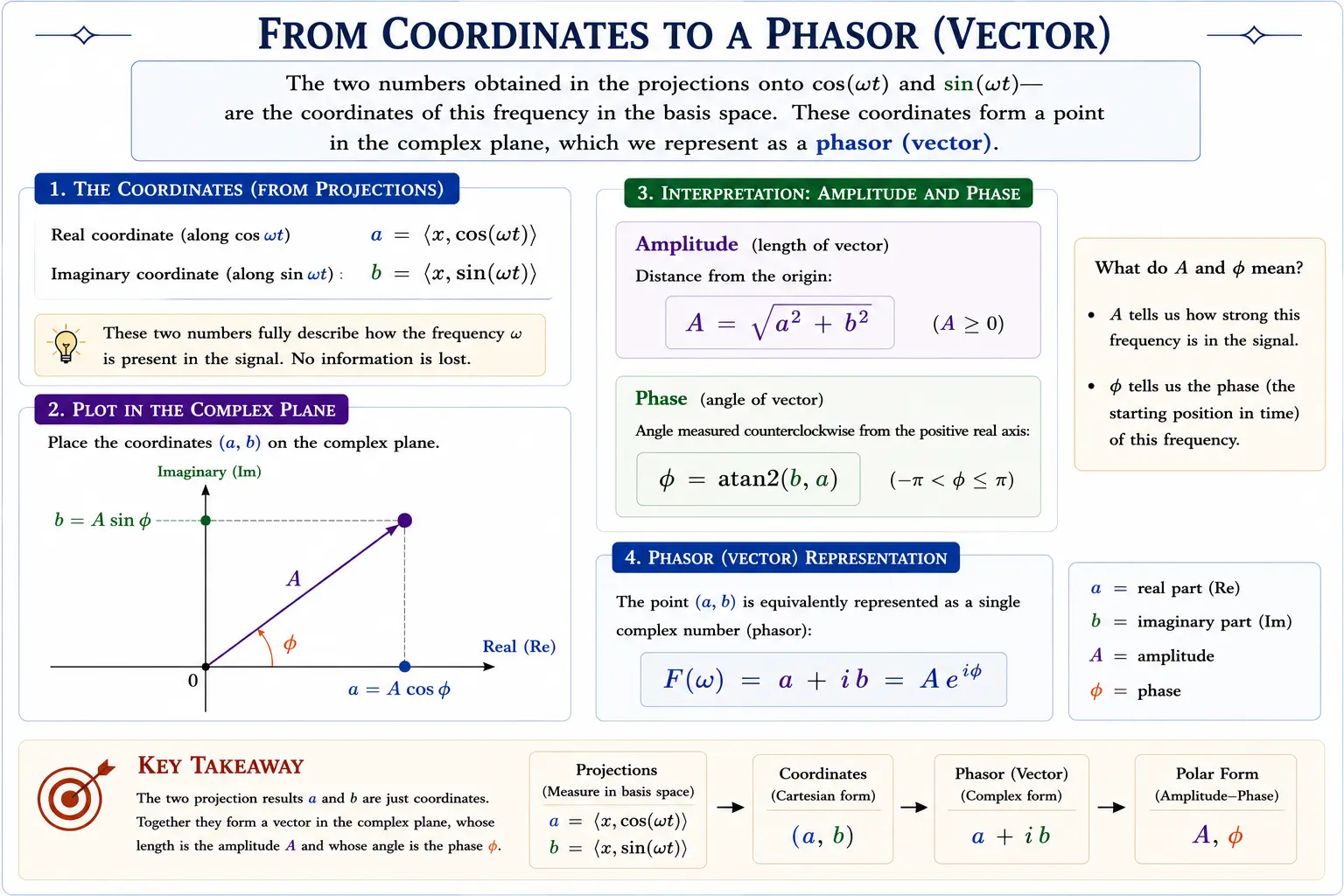
Once we have those two coordinates, everything else about the oscillation falls out almost for free. Amplitude and phase are just distance and bearing. It is interesting to notice that no new information gets created anywhere along the way; it's simply been rearranged into a shape that's actually usable. The infinite search that seemed unavoidable a little earlier has quietly disappeared, not because anyone discovered a clever shortcut through it, but because it was never really infinite to begin with. It was always just two dimensions, wearing a very convincing disguise.

Which leaves one last, slightly mischievous question hanging in the air: could those two numbers, the cosine coefficient and the sine coefficient, be thought of not as a pair, but as a single mathematical object? On the surface, that sounds like nothing more than a change in notation for its own sake. It is not. It's the doorway into complex numbers, and it turns out to be one of the more genuinely elegant turns this whole story takes.

Why bother with "imaginary" numbers?

By this point, the problem looks solved. Two orthogonal reference waves, two coefficients, done and dusted. So why do textbooks insist on dragging complex numbers into a story that seemed perfectly finished a paragraph ago?

Well, I think the honest answer is mathematicians have a long, slightly mischievous habit of swapping one perfectly valid description for another, not because the first one was wrong, but because the new one makes hard problems noticeably easier. Redrawing a map using a different projection doesn't change the actual ground beneath your feet; it just changes how convenient the numbers are to work with. In exactly the same spirit, moving a signal from the time domain into the frequency domain doesn't touch the underlying physics at all. It just reorganises the same information into a shape where oscillatory behaviour is much easier to spot. The complex plane belongs to this same family of moves, not a hidden physical dimension, but a richer language, one where certain calculations stop being awkward and start being almost easy.

We've spent considerable time analysing the oscillation itself, the measurable, real-world thing. Here's a different question worth asking: could there exist some other mathematical object, easier to manipulate than the oscillation directly, that still always reproduces the exact same observable signal whenever we need it back? If something like that existed, we could do all our actual calculations inside that friendlier object, and simply step back out into the real world whenever we wanted the measurable answer. That, it turns out, is precisely the role the complex plane is about to play.

So why does it look the way it does? Why does it need a second axis at all?

Start with an observation about multiplication that you already know but have probably never examined closely. Multiply by two, and everything doubles. Multiply by one-half, and everything shrinks. Multiply by minus one, and everything simply flips direction, which, geometrically, is a rotation of 180° about the origin. Multiplication, without anyone really noticing, has already become more than simple scaling. It's become a geometric move.

So, we add a second, independent axis: the imaginary axis, a name that has confused more people than it ever deserved to. It's simply another direction, exactly as independent from the real axis as north is from east. The terminology is historical. The geometry is entirely real.

Define a quantity, call it \(i\), as one quarter-turn within this new plane. Multiply it once: 90°. Multiply it twice: 180°, which we already know is the same as multiplying by minus one. And so:

$$i^2 = -1$$

The calculus problem: Why sine and cosine weren't enough

For every frequency, we have two basis functions, a cosine and a sine. Project the signal onto both, get two coefficients, and those two numbers describe the amplitude and phase completely. The infinite search is gone. So why keep going? Why bring in yet another mathematical language on top of everything else?

The reason to keep pushing has surprisingly little to do with oscillations themselves, and everything to do with change.

Throughout this whole article, we've been talking about signals: gravity anomalies, seismic traces, bathymetric profiles, climate records. These are all, fundamentally, measurements. But science is rarely satisfied with measurements sitting still. Science wants to know how those measurements evolve. How does temperature change over time? How does a wave propagate through the Earth? How does gravity vary across a sedimentary basin? How does stress build up and release within the lithosphere? None of these are questions about a single value. They're questions about rates of change, which is exactly why so much of physics ends up written as differential equations in the first place. The heat equation describes how temperature evolves. The wave equation describes how a disturbance propagates. Potential field theory ties spatial derivatives of physical fields together. Diffusion, elasticity, fluid flow, and a long list of other physical processes are all governed by equations built out of derivatives. Nature, in a very real sense, speaks almost entirely in the language of change.

Sine and cosine, it turns out, do remarkably well here. Differentiate a sine wave once, and you get a cosine. Differentiate that cosine, and you get minus sine. Differentiate twice more, and you're back to exactly where you started, the original sine wave, completely unchanged, having quietly toured its way through cosine and minus-sine and minus-cosine and landed right back home four steps later. That resilience is precisely what let Fourier solve the heat equation in the first place: the second derivative preserved the oscillation's identity, and only its amplitude changed, weakening as heat diffused. Without that specific, slightly stubborn behaviour, none of Fourier's original insight would have worked at all.

There's a subtle inconvenience buried in here, though. While differentiation does preserve the oscillatory character of the solution, it keeps handing information back and forth between the two basis functions, sine becomes cosine, cosine becomes minus sine, over and over. To be clear, this doesn't undo their orthogonality; that's a separate property entirely, describing how we measure the coefficients rather than how the functions behave under calculus, and it holds regardless. But from the specific angle of solving differential equations, sine and cosine start to look like two dance partners who can never quite stay still, every derivative passes the baton from one to the other. The mathematics is completely correct. It's just not as tidy as it could be.

So mathematicians, being mathematicians, naturally started wondering: is there some function that behaves even more simply under differentiation? Not merely returning to itself after two derivatives with a sign flip. Not endlessly trading identities with a partner function. Something that stays essentially unchanged every single time you differentiate it. A function like that would be extraordinarily convenient; differential equations would become dramatically easier to solve.

Unfortunately, they seem completely unsuited to what we actually need. Exponentials grow. Or they decay. Oscillations do neither. A seismic wave doesn't grow exponentially forever, a gravity anomaly doesn't decay exponentially along a survey profile, and a climate cycle bears no resemblance to a tidy exponential curve. So we appear to be stuck choosing sides: sine and cosine, because they actually describe oscillations, or exponentials, because they make the calculus so much easier. For a long time, historically, these genuinely looked like two entirely separate mathematical worlds that simply weren't going to talk to each other.

However, the mathematical plane we saw earlier where multiplication could represent rotation, was setting up the missing connection. The real question isn't "can exponentials describe oscillations?" It's something more interesting: what happens if an exponential is allowed to evolve not just along the ordinary real axis, but within this richer 'complex' plane? If such an exponential could somehow rotate instead of merely growing, the apparent conflict between exponentials and oscillations might simply dissolve. That possibility sounds almost too convenient to be real. It is, remarkably, exactly what Leonhard Euler discovered, that exponentials and oscillations were never actually rival ideas at all. They're two different descriptions of the exact same underlying thing.

The moment growing turned into spinning

Start with the exponential we already know: \(e^x\). As \(x\) grows, the function grows. As \(x\) goes negative, it decays. The exponent simply slides further along the real number line, and distance from the origin dictates how much growth or decay you get. Nothing surprising happens here at all.

However, when the exponent lives inside the complex plane, Euler showed that the exponential function stops being only about growth, and starts describing rotation too. His famous identity reads:

$$e^{i\theta} = \cos\theta + i\sin\theta$$

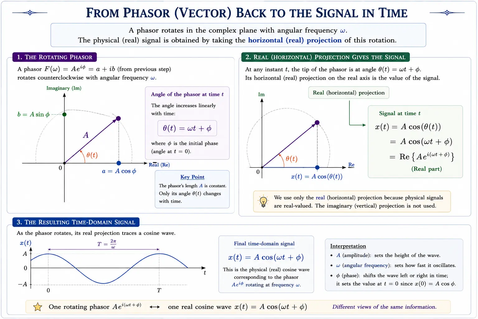
This equation should be quoted with reverence. This isn't sine and cosine magically transforming into an exponential out of nowhere. It's the revelation that all three, the exponential, the sine, and the cosine, were always the same underlying object, just described three different ways. Go back to the rotating point one final time: as the angle sweeps forward, its horizontal coordinate traces a cosine, and its vertical coordinate traces a sine. Now look at Euler's identity again: the real part of the exponential is exactly that cosine. The imaginary part is exactly that sine. The same geometry we started with, all the way back at the circle, has become an equation. What began as a mental picture is now something you can actually compute with.

Every oscillation can now be represented as a single rotating complex exponential. Every projection we've been doing onto sine and cosine separately can equally well be understood as a projection onto this one rotating exponential instead. The dance between two basis functions that kept swapping identities under differentiation gets replaced by a single mathematical object, that behaves beautifully under calculus, while simultaneously capturing amplitude, frequency, and phase.

The single-pass projection

Euler handed us something remarkable: cosine, sine, and the exponential, revealed as three faces of the same object. It's tempting to think the hard part is over. It isn't, not yet. We still haven't actually answered the question this whole search started with, all the way back when we first tried catching one wave red-handed: given a real signal, how do you actually discover which rotating exponential is hiding inside it?

We have seen the tool for this, several sections ago. To get the cosine coefficient, we multiplied the signal by \(cos(ωx)\) and added everything up. To get the sine coefficient, same move, using \(sin(ωx)\) instead. Two separate operations, two separate numbers.

Now that Euler has shown us \(cos(ωx)\) and \(sin(ωx)\) are just the real and imaginary parts of one rotating exponential, the obvious next move is to stop measuring them one at a time and project onto the exponential itself, directly, in a single pass. Multiply the signal by \(e^{i\omega x}\), and add everything up:

$$\int f(x)\, e^{i\omega x}\, dx \;=\; \int f(x)\cos(\omega x)\, dx \;+\; i\int f(x)\sin(\omega x)\, dx$$

Which is just the cosine coefficient sitting quietly in the real part, and the sine coefficient sitting in the imaginary part, both produced by a single integral instead of two separate ones done by hand.

The Fourier Transform, at last

We've come a fairly long way to get here. We started with a hot iron rod in a nineteenth-century forge, and discovered that heat smooths temperature variations out, favouring the long and gentle over the short and sharp. We found out why sine waves survive differentiation with their identity intact. We imagined a point going round and round a circle and found frequency, amplitude, and phase quietly hiding in its shadow. We used arithmetic to measure resemblance between waveforms using nothing more than multiplication and addition. We swapped an infinite search over every possible phase for two fixed, orthogonal coordinates. We saw how a second mathematical direction make rotation possible. Then Euler showed us that exponentials and oscillations had been describing the same thing all along. We also learned how to project a signal onto a single rotating exponential, instead of two sinusoids.

Of course, the Earth was never going to restrict itself to a single frequency out of politeness. A seismic trace might contain hundreds. A gravity profile might span structures across dozens of different wavelengths. A climate record might hide several overlapping periodicities layered on top of each other. So we just repeat the exact same procedure, over and over: choose another frequency, build another reference, project, measure, record the result. Again. And again. Each repetition is asking precisely the same narrow question: how much of this particular oscillation is actually present in the data? The full collection of all those answers, gathered together, is what we call the Fourier Transform.

Which finally lets us write down the equation itself:

$$F(\omega) = \int_{-\infty}^{\infty} f(x)\, e^{-i\omega x}\, dx$$

There's a small, deliberate wrinkle worth flagging here, because it explains something that would otherwise look arbitrary at the moment. The "convention" is that the signal gets projected onto \(e^{-i\omega x}\) instead of \(e^{i\omega x}\). It is the same rotation, just running the other way, which only flips the sign in front of the sine coefficient. Nothing deep is happening.

I believe every single symbol here has already shown up somewhere in this article, wearing a different hat. \(f(x)\) is just the measured signal. \(e^{-i\omega x}\) is the rotating reference oscillation, with its frequency set by \(\omega\) and its spin direction fixed by the "convention" we just mentioned a moment ago. The multiplication and the integral together are exactly the single-pass projection we just built, stretched out now to run over the entire signal rather than one instance of it. And \(F(\omega)\) is simply the coordinate of the signal at that particular frequency, nothing more mysterious than projecting a vector onto a coordinate axis, except that here, the axes happen to be oscillations instead of arrows.

Now, there are some loose threads that requires tying off properly. Normalization. Should the size of the coefficients depend on how long the signal happens to be? Should doubling the number of samples double every coefficient along with it? Obviously not, so different fields have settled on different conventions for exactly where to put the scaling factor. Some tuck it into the forward transform. Some put it in the inverse transform instead. Others split it evenly across both. None of these choices touches the underlying physics in the slightest; it's the exact same situation as kilometres versus miles describing the identical distance with different numbers attached. This single point, once you see it, explains why two perfectly correct software packages can hand you spectra that look numerically different while meaning exactly the same thing underneath.

Also the equation above quietly assumes the signal is known continuously, across all of space or all of time, forever. Real data is never remotely like that. Seismic traces are sampled at discrete intervals. Gravity measurements come from a finite set of stations. Bathymetric surveys are made of a finite number of soundings. Climate records are built from individual, discrete observations. Computers, at the end of the day, work with finite arrays of numbers, never with smooth continuous functions. Does any of that undo everything we've just learned? Not at all. The underlying philosophy stays exactly the same; only the mathematics adjusts slightly to fit. The continuous integral becomes a finite sum. The infinitely many possible positions become a finite set of discrete samples which introduces some attributes of its own. The continuous Fourier Transform becomes the Discrete Fourier Transform, and because even that sum can get computationally expensive while dealing with real datasets, another idea eventually showed up to make it fast: the Fast Fourier Transform.

Fast Fourier Transform is, regretfully, where I actually entered this entire story, years before I understood a single thing that came before it. One line of code, fft(signal), hit enter, and a spectrum appears looking like a magic trick (of course, not instantly, seeing the spectrum often requires some more lines of code). However, underneath that one line of code sits this entire journey, compressed down into microseconds: a computer quietly asking, over and over, thousands of times, millions of times, "how much of this oscillation is actually here?"

It's also worth being precise about what the Fourier Transform actually does, and, just as importantly, what it doesn't. The Fourier Transform does not invent oscillatory structure that is absent from the data. It expresses the signal in a sinusoidal basis, nothing more. Whether a given spectral peak corresponds to a genuine, distinct physical process, or instead arises from interference between nearby frequencies, the finite length of the observation, windowing, or some other artefact of the measurement itself, remains a matter of interpretation, not something the mathematics settles on its own. That job still belongs entirely to us, 'Humans'. A spectral peak, sitting there on its own is just evidence, nothing more, and its real significance depends completely on which geological, geophysical, or climatic process is actually capable of producing a signal at that particular scale, once the more mundane explanations have been ruled out. The mathematics hands us the coordinates. Figuring out what they actually mean is still our job, which is often the more interesting half of the work.

How computers actually pull this off efficiently, what assumptions sneak in along the way, and why spectra sometimes genuinely mislead you if you're not careful, that's the Discrete and Fast Fourier Transform, and it's a story for another day.

Arjun

Please feel free to leave your comments and suggestions...

• 
• 
• 
• 
• 
•